


This is for newcomers to ML who want to start easy, and then step up
Easy to large
This post is for newcomers to ML who have learned to work with Jupyter Notebooks and now want to know: How do I move up to a production-ready system using AWS services?
You’ve started lightweight and local, but and now you need to get to the distributed systems that can handle the heavy loads like:
- Glue for transformation and metadata catalog
- Athena for direct queries into S3 buckets
- QuickSight for visualization of analytics
- Sagemaker Instances for parallelized training
- Sagemaker Endpoints for versioned, autoscaled inference servers
Start from Notebooks
Jupyter Notebooks are a wonder for Machine Learning, an online IDE that maintains the state of local variables in memory so you can work with the kind of long-running process that is ML. Sagemaker Notebooks (Console; Docs) give you a managed environment to quickly spin these up. You can do everything there, including loading data, exploring, preprocessing, visualizing, training, evaluating, and deploying — all in a single memory-space for convenience and speed.
Distributed AWS services
Beyond the Notebook, it gets harder: You have to coordinate a series of heavyweight distributed services, integrating each part, making sure they authenticate to each other.
It’s hard to keep a clear understanding of what is happening across the ML process. First, because the state of the process is distributed (mostly in S3 buckets), and second, because of the long waits while AWS services are triggered and large amounts of data are processed.
In this post, I’ll explain how to make that move, gradually.
Making the move
A single interactive environment is no way to run production systems. At some point, you need to move from the Notebook to that distributed system.
I’d like to give an example of how to break each piece out as you move up the continuum towards a production system. We’ll illustrate with this open-source Notebook. In this article, you can see how to step through it in a Sagemaker Notebook instance — or even more easily, in the new Sagemaker Studio (Console; Docs). For each type of functionality, I pull out a snippet or two of code from the Notebook, then compare it to the distributed system that provides the same functionality inside AWS. In some cases, that Notebook already uses AWS, by invoking Sagemaker for training and deployment; for such cases, I explain how you would step up from simple local execution to the Sagemaker APIs, and beyond to a system orchestrated outside the Notebook.
Ingestion
Getting the data into your system is the first step.
In a Notebook
In a Notebook, you just load a CSV or other file straight into your disk, for processing in memory.
#
From the example Notebook
with zipfile.ZipFile('bank-additional.zip', 'r') as zip_ref: zip_ref.extractall('.')
With AWS Services
With large-scale projects, local resources in your small Notebook instance would be overwhelmed.
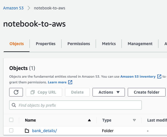
Instead, take the CSV, or other data, and put it in an S3 bucket (Console; Docs) representing the origin of your data. For static data sources, put it straight into S3; for ongoing ingestion of data by streaming, use Kinesis (Console; Docs) to output into S3.
Schemas
Next is schema identification: You have a large blob of (what looks from the outside like) unstructured data, and you want to be able to query and manipulate it according to its internal structure (generally a tabular row-and-column format).
In a Notebook
In the Notebook, the schema is automatically identified from the CSV header row when it is loaded into a Dataframe.
#
From the example Notebook
data = pd.read_csv(‘./bank-additional/bank-additional-full.csv’)
With AWS Services
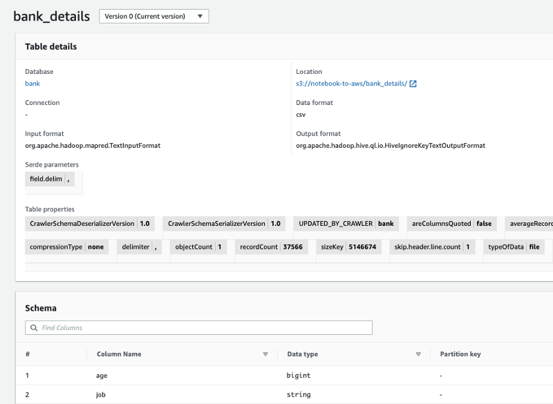
In AWS, create a Glue Crawler (Console; Docs) to identify the schema of this CSV from its column headers.
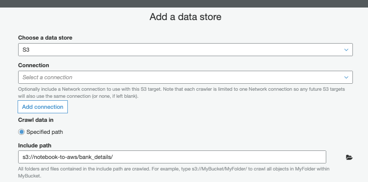
Glue Crawler inserts the schema into the Glue Data Catalog (Console; Docs). In upcoming steps (see below), Athena, Databrew, Quicksight, and other services will be able to treat these S3 objects as structured data.
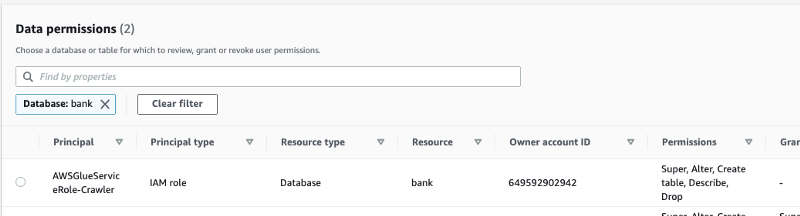
Lake Formation (Console; Docs) then controls access to these Data Catalog tables.
Exploratory Data Analysis
Next, you discover patterns in the data and transform it to make useful ML input.
In a Notebook
Even in production scenarios, you can accomplish a lot by using a manageably-sized randomly sampled subset of data and exploring it in a Notebook.
With Pandas, for example, you can understand the frequency distributions.
# From the example Notebook for
column
in
 data.select_dtypes(include=[‘object’]).columns:
    display(...)
Visualization makes good use of the human brain’s visual processing centers to highlight patterns. You can visualize the data in a Notebook, creating histograms, heat maps, scatter matrices, etc. using Seaborn and other libraries.
# From the example Notebook
for column in data.select_dtypes(exclude=['object']).columns:
   ...
   hist = data[[column, 'y']].hist(by='y', bins=30)
   plt.show()
# From the example Notebook
pd.plotting.scatter_matrix(data, figsize=(12, 12))With AWS services
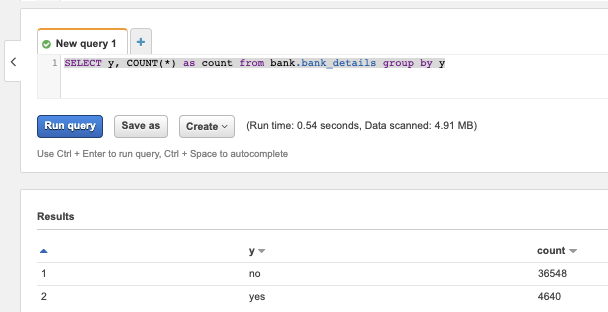
In AWS, Athena (Console; Docs) lets you directly explore the full data with good ol’ SQL. Athena uses the schema saved in Glue Data Catalog to query against the structure in the S3 objects.
For visualization of data, use Quicksight (Console; Docs), directly on top of your Athena queries. These visualizations have the advantage of being easily shareable with other people, for example, business analysts, who can contribute insights.
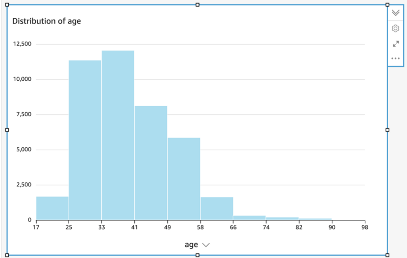
QuickSight created this histogram automatically when pointed at the age column
Transformation
In a Notebook
In your Notebook, you use the insights from EDA to transform data into a form usable as input for your training algorithm, using APIs that work with Pandas Dataframes:
- normalization for numerical data
- one-hot encoding for categorical data
#
From the example Notebook
# Convert categorical variables to sets of indicators
# (One-hot)
model_data = pd.get_dummies(data)
- arithmetic functions like multiplication and modulus
- dropping columns
#
From the example Notebook
model_data = model_data.drop([‘duration’, ...], axis=1)
- dropping outliers
- string manipulation
- and more
You then convert the data into a format that allows faster ML, such as Parquet or libsvm.
With AWS Services
Scaling up, AWS gives you several different tools for transformation:
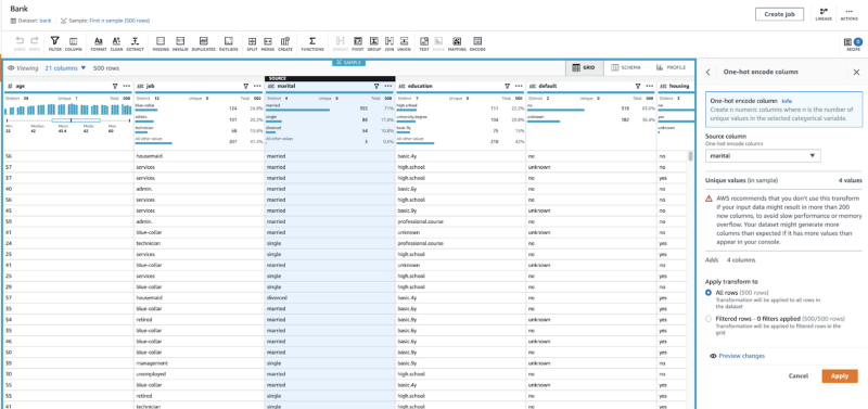
DataBrew (Console; Docs) is a graphical transformation builder — one of the few in my experience that works well. It reads your S3 data, as defined in the Glue Data Catalog. You choose from a selection of transformations like one-hot, normalization, and others that I listed above in the context of Notebooks.
DataBrew generates transformations that run in the Glue framework. As a last step in the transformation, the data can be converted into the desired ML format like Parquet, Avro, CSV, or JSON.
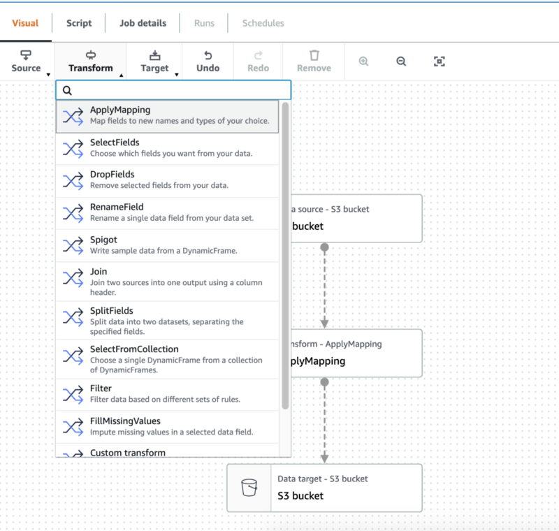
Alternatively, Glue Studio (Console; Docs) gives you a graphical transformation tool —though without DataBrew’s ML-oriented transformations such as one-hot — and you can write your own Python or Scala transformation code to be run in Apache Spark.
Training
Without Sagemaker
You may be running algorithms like XGBoost directly in the memory of your Notebook. This is good for interactive rapid development.
See, for example, this non-Sagemaker local invocation of XGBoost.
#
From a Notebook that does not use Sagemaker
from xgboost import XGBClassifier # Non-Sagemaker package
...
model = XGBClassifier(… )
...
model.fit(...)
With Sagemaker
As it happens, our sample Notebook is already set up to invoke the Sagemaker SDK (Docs), and if you are not doing that, it is your easy next step. The API here is the same as for other open-source libraries that run the same algorithm — you just need to import a different library.
#
Using Sagemaker (from the example Notebook
)
from sagemaker.estimator import Estimator # Different package
...
xgb = Estimator...
...
xgb.fit(...) # Same API
The Sagemaker SDK allows both local and remote training: You can train in local mode for fast iteration during development (you may have been doing before), but then, as you scale up, you use the SDK to trigger training on specialized Sagemaker instances (Console; Docs), including powerful features like distributed training on multiple instances.
With the same SDK, you can also call the algorithms with hyperparameter tuning (Docs): The same algorithm is run multiple times, each with a different set of parameters, looking for the parameters that give the same results.
Deployment and Evaluation
Without Sagemaker
If you are training locally, without Sagemaker, then you don’t need to deploy at all: You run inference right inside your memory space. For example, you might evaluate performance by running your inferencing (predict()) on a hold-out set.
#
From a Notebook that does not use Sagemaker
y_pred = model.predict(X_test) # XGBClassifier model created above
...
pd.crosstab(…) # Evaluate confusion matrix using Pandas
With Sagemaker
In Sagemaker, you’ll want to deploy to an Endpoint, a set of instances that responds to inference requests (Console), as is done in our sample Notebook.
#
Using Sagemaker (from the example Notebook
)
xgb_predictor = xgb.deploy(…) # Using Estimator created above
For scaling, you can add more inferencing instances, or configure them to autoscale, and you can call on more computing-power-as-a-service with Elastic Inference.
When you redeploy a new version of the model, you compare its performance on a new endpoint, using Sagemaker’s support for A/B testing.
Invoke inference in the endpoint with predict() , just as in the non-Sagemaker code. You can evaluate results by inferencing on a hold-out set, and then calculating metrics with Pandas and other in-memory APIs.
#
Using Sagemaker (from the example Notebook
)
xgb_predictor.predict(…)
pd.crosstab(…) # Evaluate confusion matrix using Pandas
But that’s in a Notebook!
Our goal was to get off the Notebook and into the AWS scalable systems, so you might be wondering why the last few stages were still in a Notebook.
On the one hand, these key steps did in fact invoke Sagemaker distributed APIs, rather than running in-process, so are fully scalable. In a basic workflow, where you occasionally retrain and redeploy the model by hand, they might even be workable for a manual, non-automated system.
On the other hand, in a typical ML production process, new versions of the model must be retrained and redeployed continually, just as you build and test your software with a Continuous Integration/Continuous Deployment pipeline. For this, you define your directed acyclic graph of ML processing steps in JSON, including, for example, data-cleaning, pre-processing, training, deployment, and evaluation APIs. (Here is a useful example for setting up a Pipeline.) You can reuse your existing code as the code in the Notebooks is just Python and can run anywhere, even in a pipeline.
A Notebook is a powerful tool for development, but as you move into production, you will want more powerful infrastructure. This article shows you how to carve pieces out, one by one, even allowing you to continue working with the Notebook while also letting the main system run autonomously.
I hope this post has helped you step up to large production systems.
— — —
P.S. This post is based on my AWS AI/ML Black Belt experience, an advanced certification that goes beyond the test-based AWS Certified ML Specialty. The Black Belt includes an advanced course and a final Capstone project which is the basis for your certification. It’s a great way to build and then show your skills in the areas mentioned above. See a more detailed post about it here.
Thanks for reading! To stay connected, follow us on the DoiT Engineering Blog, DoiT Linkedin Channel, and DoiT Twitter Channel. To explore career opportunities, visit https://careers.doit.com.